Exp 1 dtsp pole zero
%Exp1:Pole-zero plot & freq response
clc;
clear all;
close all;
%Take TF as input
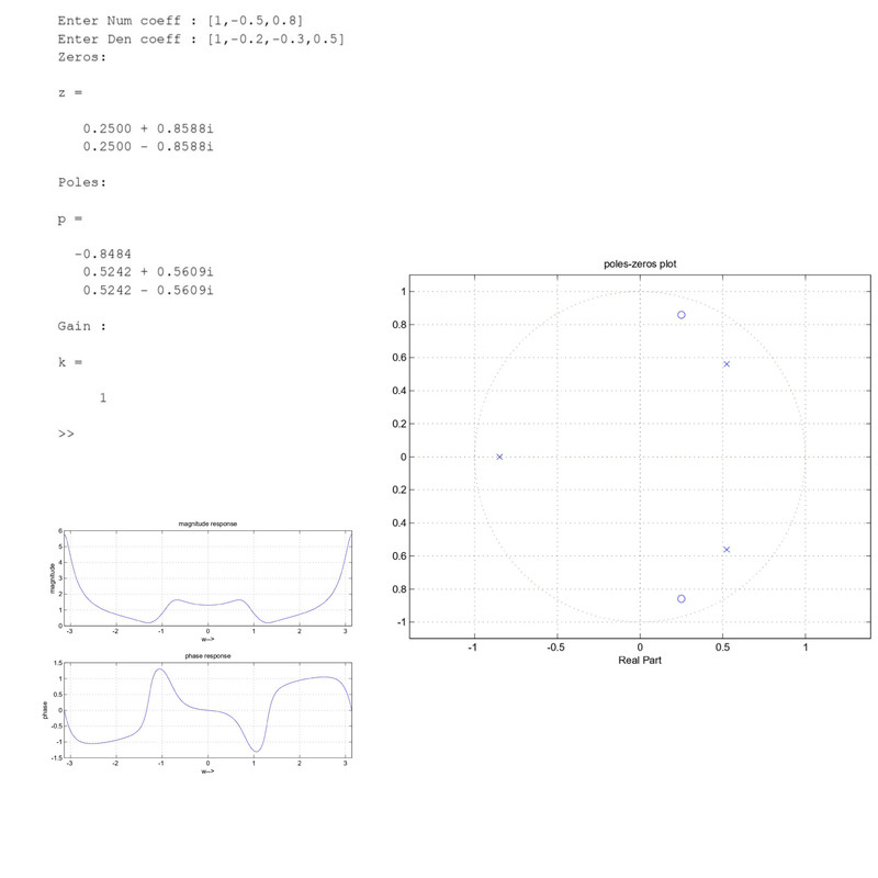
N=input('Enter Num coeff : ');
D=input('Enter Den coeff : ');
%Find poles-zeros
[z,p,k]=tf2zp(N,D);
disp('Zeros: ');z
disp('Poles: ');p
disp('Gain : ');k
%poles-zero plot
figure;
zplane(z,p);grid on;
title('poles-zeros plot');
%Frequency Response
W=-pi:0.001:pi;
H=freqz(N,D,W);
Hmag=abs(H);
Hphase=angle(H);
figure;
subplot(2,1,1);
plot(W,Hmag);grid on;
xlim([-pi,pi]);
xlabel('w-->');
ylabel('magnitude');
title('magnitude response');
subplot(2,1,2);
plot(W,Hphase);grid on;
xlim([-pi,pi]);
xlabel('w-->');
ylabel('phase');
title('phase response');
EXP 1 OUTPUT
Exp 2 convolution and correlation
%Exp2.1:Convolution and correlation
clc;
clear all;
close all;
%%Convolution
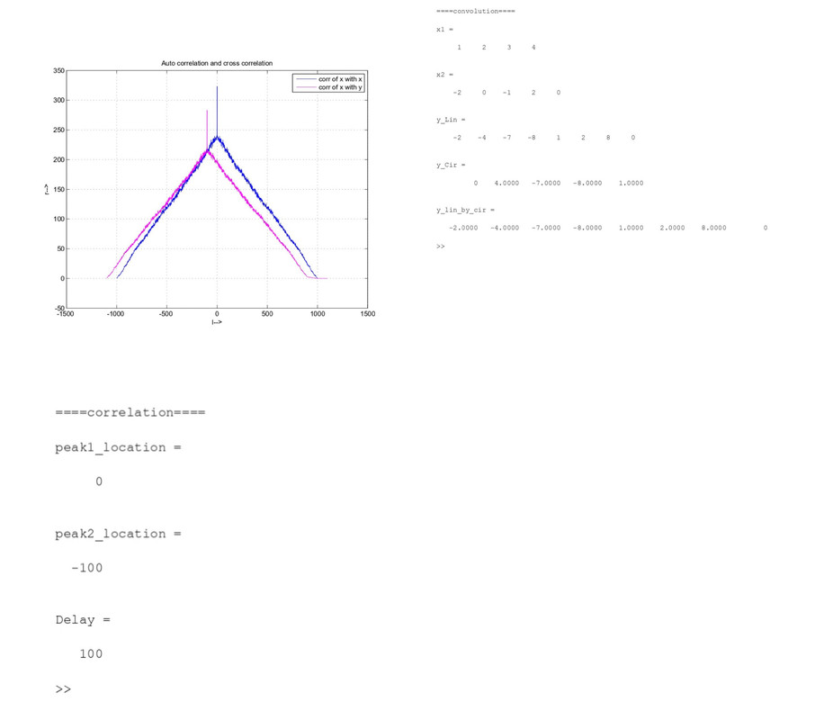
disp('====convolution====');
x1=[1,2,3,4]
x2=[-2,0,-1,2,0]
L1=length(x1);
L2=length(x2);
%Linear convolution
y_Lin=conv(x1,x2)
%Circular convolution
L=max([L1,L2]);
y_Cir=cconv(x1,x2,L)
%Linear conv using circular conv
N=L1+L2-1;
pad1=N-L1;
pad2=N-L2;
x1_pad=[x1,zeros(1,pad1)];
x2_pad=[x2,zeros(1,pad2)];
y_lin_by_cir=cconv(x1_pad,x2_pad,N)
%Exp2.2:Convolution and correlation
clc;
clear all;
close all;
%%Correlation
disp('====correlation====');
%x=[1,2,3,4]
%y=[0,0,1,2,3,4]
x=rand(1,1000);
y=0.8*[zeros(1,100),x]+0.1*rand(1,1100);
%y=[x,zeros(1,100)]+0.5*[zeros(1,100),x];
%Auto correlation of x
[r_xx,l_xx]=xcorr(x,x);
%cross correlation of x with y
[r_xy,l_xy]=xcorr(x,y);
%plot autocorrelation & cross correlation
figure;
plot(l_xx,r_xx);
grid on;
hold on;
plot(l_xy,r_xy,'m');
legend('corr of x with x','corr of x with y');
title('Auto correlation and cross correlation');
xlabel('l-->');
ylabel('r-->');
%To find peak location
[max_xx,I_xx]=max(r_xx);
peak1_location=l_xx(I_xx)
[max_xy,I_xy]=max(r_xy);
peak2_location=l_xy(I_xy)
Delay=abs(peak1_location-peak2_location)
EXP 2 OUTPUT
Exp 3 Truncation of ideal impulse
clc;
clear all;
close all
;
%take input
wc=input('enter cutt of frequency:');
N=input('enter truncation limit:');
%find n
nn=
-N:
-1;
nz=0;
np=1:N;
n=[nn,nz,np];
%find hid(n)
hid_n =sin(nn*wc)./(nn*pi);
hid_z
= wc/pi;
hid_p =sin(np*wc)./(np*pi);
hid=[hid_n,hid_z,hid_p];
%display imp res
figure;
stem(n,hid);
xlabel('n-->');
ylabel('hid(n)-->');
title('truncated ideal imp res');
%Frequency Response
w=
-pi:0.001:pi;
H=freqz(hid,1,w);
Hmag=abs(H);
Hphase=angle(H);
figure;
Subplot(2,1,1);
plot(w,Hmag); grid on
; Xlim([
-pi,pi]);
xlabel('W-->'
)
ylabel('Magnitude');
title('Magnitude Response');
subplot(2,1,2);
plot(w,Hphase); grid on
; Xlim([
-pi,pi]);
Xlabel('W-->'),
Ylabel('Phase');
title('Phase Response'
)
Exp. 4: Filter Realization
clc;
clear all;
close all
;
%Define filter coefficients
b=[1,1/3];
a=[1,
-3/4,1/8];
%Display TF
fs=1;
H_z=tf(b,a,fs,'variable'
,'z^
-1');
disp('Transfer Function');H_z
%%Direct Form
1
%create filter object
H_df1=dfilt.df1(b,a);
info(H_df1);
%Realization
realizemdl(H_df1);
%%Direct Form
2
%create filter object
H_df2=dfilt.df2(b,a);
info(H_df2);
%Realization
realizemdl(H_df2);
%%Cascade Form
%Define H1(z)
b1=[1,1/3];
a1=[1,
-1/2];
H1=dfilt.df2(b1,a1);
%Define h2(z)
b2=[1];
a2=[1,
-1/4];
H2=dfilt.df2(b2,a2);
%Create Cascade Object
H_cascade=dfilt.cascade(H1,H2);
info(H_cascade);
%Realization
realizemdl(H_cascade);
%%Parallel Form
%Define H3(z)
b3=[10/3];
a3=[1,
-1/2];
H3=dfilt.df2(b3,a3);
%Define h4(z)
b4=[
-7/3];
a4=[1,
-1/4];
H4=dfilt.df2(b4,a4);
%Create parallel Object
H_parallel=dfilt.parallel(H3,H4);
info(H_parallel);
%Realization
realizemdl(H_parallel);
Exp 5convolution using dft idft
clc;
clear all;
close all;
%Define inputs
x=[1,2,3,4]
h=[2,-1,3]
L1=length(x);
L2=length(h);
%%Circular convolution
disp('==== Circular convolution ====');
N=max(L1,L2);
y_cir_direct=cconv(x,h,N)
X_k=fft(x,N)
H_k=fft(h,N)
Y_k=X_k.*H_k
y_cir_DIFT=ifft(Y_k,N)
%%Linear convolution
disp('==== Linear convolution ====');
L=L1+L2-1;
y_lin_direct=conv(x,h)
X_k=fft(x,L)
H_k=fft(h,L)
Y_k=X_k.*H_k
y_lin_DIFT=ifft(Y_k,L)
Exp 6 freq analysis using data
%EXP6:FREQUENCY ANALYSIS USING DFT
clc,clear all,close all;
%load data
load('Data.mat');
%x=x+0.2*sin(2*pi*200*t);
%DISPLAY DATA
figure;
plot(t(1:100),x(1:100));
title('Given Signal');
%play Sound
%sound(x);
%disp('Press any key to play given signal');
%pause();
%Find DFT of Signal
N=2048;
Xk=fft(x,N);
%DISPLAY SPECTRUM
Xk_mag=abs(Xk);
figure;
plot(Xk_mag);
title('Spectrum (DFT) of signal');
%Find Location of Peaks
[peaks,Location]=findpeaks(Xk_mag(1:N/2),'SortStr','descend','Npeaks',3)
k=Location-1
%Frequency corresponding to k
f=k*fs/N
 Exp 2 convolution and correlation
 Exp 3 Truncation of ideal impulse